How NASA Uses Artificial Intelligence to Detect Exoplanets

Houston, I want to believe!

Being just a tiny blue dot in the ever-expanding universe, humans of Earth have been wondering for centuries if they are alone here. The answer to this question is the motivator behind scientific research of the world’s best minds, exquisitely equipped observatories, neatly designed spacecrafts, and the rapidly developing and emerging technologies.

To get the answer, other planets, naturally, first have to be discovered. Any planet is just a faint source of light in comparison to the parent star it is orbiting. For instance, the Sun is a billion times as bright as the reflected light from Earth or Mars, or any of the other planets in our solar system. This gives astronomers a double trouble of identifying an exoplanet that provides a hard-to-distinguish source of light, which is outwashed by a powerful glare of the parent star at the same time.

William Fawcett

Due to this reasons, very few extrasolar planets can be observed directly, and even fewer can be distinguished from its parent star. As of September 27, 2018, there were 3,791 confirmed exoplanets, most of which were detected by the Kepler spacecraft. For instance, there were 1,300 exoplanets found in 2016.

At the recent TensorFlow meetup in London, William Fawcett of the NASA Frontier Development Lab shared insights to how the institution uses artificial intelligence to find life beyond Earth.

“The galaxy is very big, I’m sure you’re all aware. There is something like 100 billion stars, and we think about 40 billion of those stars have a planet orbiting it that could potentially host life.” —William Fawcett, NASA Frontier Development Lab

Using transit methods to detect an exoplanet

Exoplanets can be detected using the transit techniques, which imply measuring the brightness of a target star as a function of time, producing a flux time series called a light curve. Simply put, exoplanets are detected when they transit in front of a star like our Sun and cause a drop in the measured brightness.

Stars transiting in front of the Sun (Image credit)

However, the signals of such a star passing are hardly traceable in comparison to the instrumental noise and systematics, as well as the inherent stellar variation present in the data captured and measured. In addition, such false-positive planet signals as background eclipsing binaries, for example, should be removed to achieve a reliable result. With all the massive data sets of light curves produced by Kepler and other spacecrafts sailing the universe, scientists need efficient means of processing and analyzing the data. This is where machine learning comes helpful.

“Detecting an exoplanet is as tricky to spot as a firefly flying next to a searchlight from thousands of miles away.” —William Fawcett, NASA Frontier Development Lab

Detecting an exoplanet is still just a beginning of the mission. Now, the scientists have to find some evidence of life to label the planet as the one potentially hosting life. The next step is measuring atmospheric spectrum, which is essential to understanding what a planet’s size and atmospheric properties are. The method underlying such findings is transmission spectroscopy.

When a planet passes the parent star, it blocks a fraction of the stellar flux equal to the sky-projected area of the planet relative to the area of the star. The fractional drop in flux is referred to as the transit depth. The main idea behind transmission spectroscopy is that the planet’s transit depth is wavelength-dependent. At wavelengths where the atmosphere is more opaque due to the absorption by atoms or molecules, the planet blocks a bit more of stellar flux. To measure these variations, the light curve is binned in wavelength into spectrophotometric channels, and the light curve from each channel is fit separately with a transit model. The measured transit depths as a function of wavelength constitute the transmission spectrum.

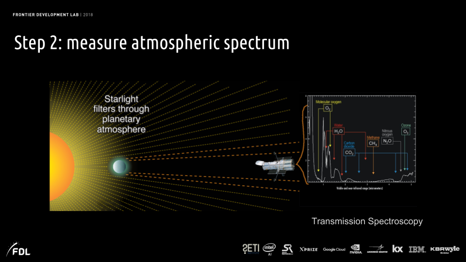Using transmission spectroscopy to measure atmospheric spectrum (Image credit)

Then, it is time to retrieve the atmospheric parameters like temperature, pressure profile, atmospheric density, composing elements, etc. from spectrum. These are the biohints suggesting the planet is fit for life. For instance, the atmospheres’ temperature provides an indication of the temperature at the surface. So, if the planet has the right temperature, there may be liquid water, which is one of the major requirements for hosting human-like life.

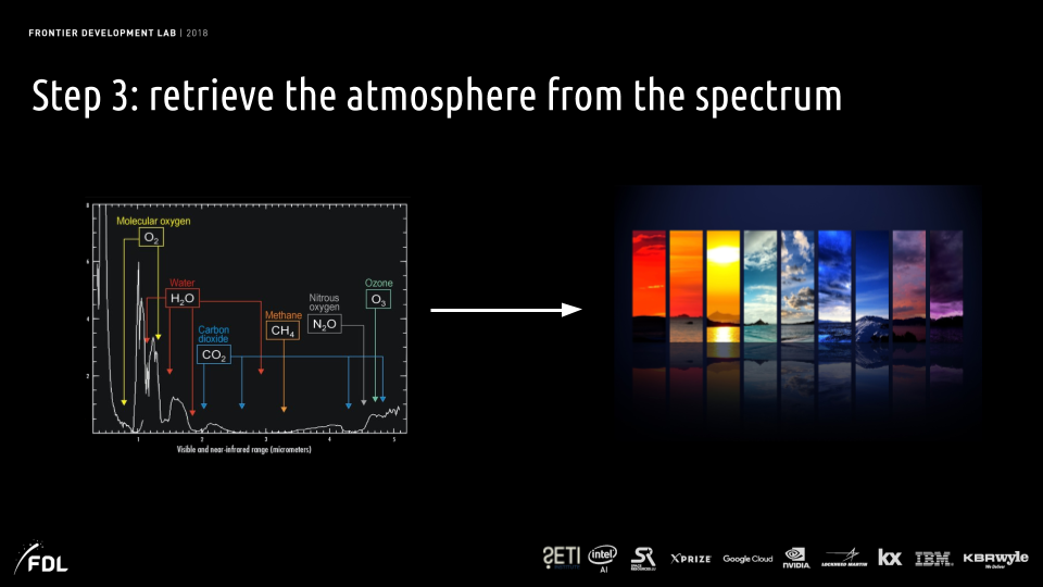Retrieving atmospheric properties from spectrum (Image credit)

These steps are challenging by themselves, and extra trouble adds up as no real data is available, so scientists have to find means to generate it, as well as processing and analyzing the data is computer-intensive. So, what’s the next move then?

Planetary Spectrum Generator

To address the lack of real data, scientists at NASA use machine learning to generate it. To be more specific, NASA has a tool of its own—Planetary Spectrum Generator (PSG)—which provides a three-dimensional orbital calculator for most bodies in the Solar system and all the confirmed exoplanets. PSG is capable of calculating any possible geometry parameters needed when computing spectroscopic fluxes. The astronomical data is based on pre-computed ephemerides tables that provide orbital information from 1950 to 2050 with a precision of a minute.

The PSG tool performs the numerical integration of the orbit by extracting orbital parameters from the NASA Exoplanet Archive. Due to the uncertainty and degeneracies in the derivation of the orbital parameters for exoplanets, PSG assumes the following:

• The longitude of ascending node (Ω) is assumed to be π.
• The planets are tidally locked, and the star sub-solar latitude/longitude are set to the center of the planet.
• The phase identifies the true anomaly with respect to that of the secondary transit, with a phase of 180 degrees corresponding to the primary transit.

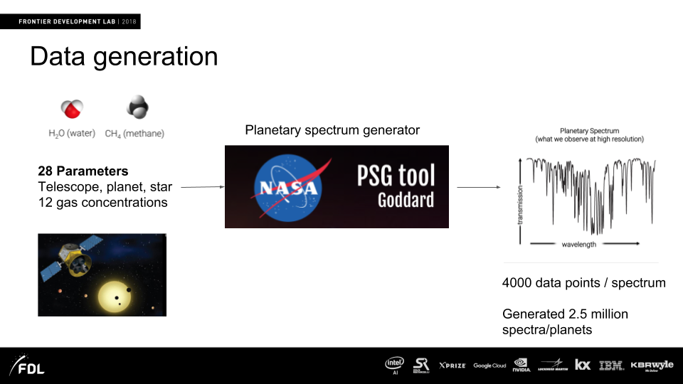NASA uses its PSG tool to generate data (Image credit)

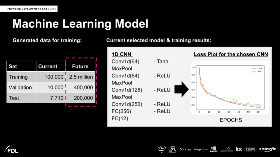
To get a working model to be further used for training, scientists also apply linear regression, as well as feedforward and convolutional neural networks. After that, model grid search, selection, and tuning are conducted before the model is ready for training. William shed some light on the grid search parameters set, which are the following:

• learning rates: 0.0001, 0.001, 0.01
• optimizers: ADAM, SGD, ADAdelta, RMSProp
• activation functions: Tanh, Softmax, ReLU, ELU, Linear

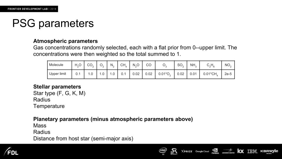The parameters supported by the PSG tool (Image credit)

So far, the team at NASA was able to generate around 100,000 data points for for training, 10,000 for validation, and around 7,710 for testing sets. This amounts to 2.5 million spectra at the training stage, 400,000 for validation, and 200,000 for testing.

Generating spectra data (Image credit)

As William explained, in the exemplary results below, one can see atmospheric properties(on the right)—how much water and methane is there—generated for a single planet. The black lines indicate the prediction made through training a model, while the red lines indicate the real situation. As far as one can see, the results are quite matching. The closeups on the left give a more detailed insight into prediction vs. reality.

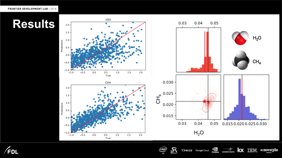The results of generating spectrum data (Image credit)

In this GitHub repo, you will find a Python package for interacting with the Planetary Spectrum Generator.

INARA: Intelligent Exoplanet Atmosphere Retrieval

William also shared some information about another tool employed by NASA researchers—INARA, which stands for intelligent exoplanet atmosphere retrieval. This tool is used to generate spectra of rocky planets and to train a machine learning model for retrieving atmospheric parameters.

INARA produces high resolution spectra and then saves observation simulation for the requested number of randomly generated planets across the parameters set. This mode allows for saving data for learning, validating, and testing a model. The generated spectra (observation simulations) can be used to train a machine learning model as a single one or in an ensemble mode.

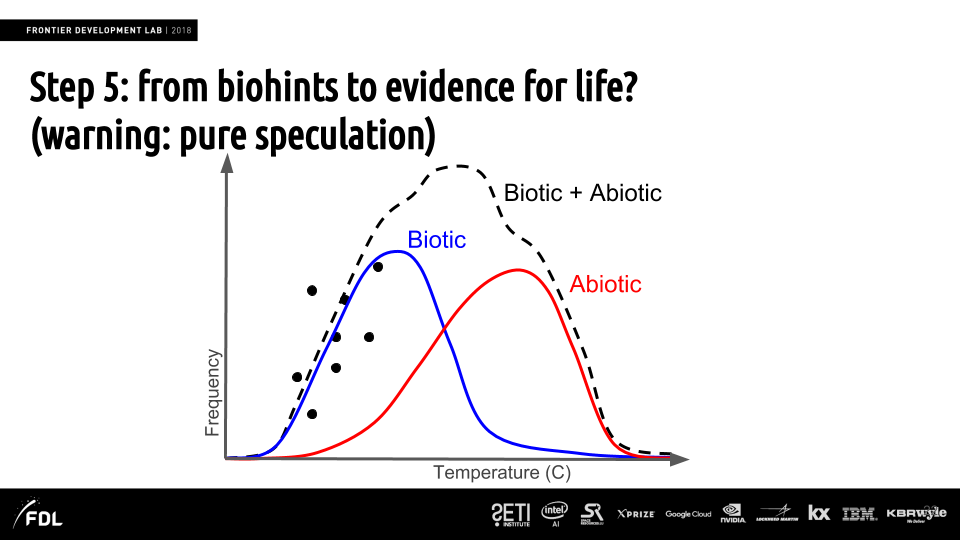Finding biohints to confirm an exoplanet as the one hosting life (Image credit)

There is also a possibility to instantiate virtual machines (VMs) to either generate planetary spectra or use the above-mentioned PSG tool on the Google Cloud. The VMs are instantiated on hard-coded parameters loading Docker images and running the command-line parameters. You can check out how to install the tool and use it for different scenarios through its GitHub repo.

You can also make use of this cheat sheet, which provides a quick introduction to classifying exoplanet candidates with machine learning.

Want details? Watch the video!

Related slides

Further reading

• Analyzing Satellite Imagery with TensorFlow to Automate Insurance Underwriting
• Digital Twins for Aerospace: Better Fleet Reliability and Performance
• What Is Behind Deep Reinforcement Learning and Transfer Learning with TensorFlow?

About the expert

William Fawcett is a researcher with a PhD in Particle Physics from the University of Oxford. He is skilled in data science, mathematical modeling, machine learning, and computer programming. William was engaged as a researcher in the NASA Frontier Development Lab, which is an 8-week applied artificial intelligence research accelerator established to maximize new AI technologies and capacities emerging in academia and in the private sector—to apply them to challenges in the space sciences. William also serves as a research team leader at CERN, where he is involved in the analysis of LHC data for new physics. In his research, William makes use of data reduction techniques to deal with large data volumes (100 TB).