Implementing Linear Regression with TensorFlow
Introduction
Linear regression helps to predict scores on the variable Y from the scores on the variable X. The variable Y that we are predicting is usually called the criterion variable, and the variable X that we are basing our predictions on is called the predictor variable. If there is only one predictor variable, the prediction method is called simple regression.
Prerequisites
In addition to TensorFlow, install Matplotlib for using plots: pip install matplotlib.
A data set
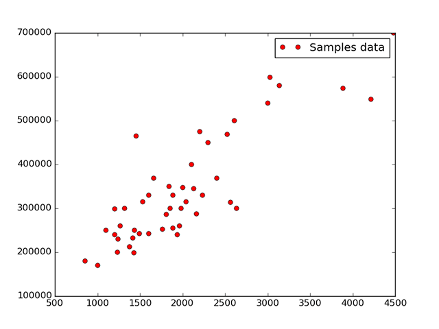
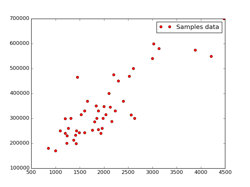
As a training set for the tutorial, we use house prices in Portland, Oregon, where X (the predictor variable) is the house size and Y (the criterion variable) is the house price. The data set contains 47 examples.
Data set pre-processing
Normalizing your data helps to improve the performance of gradient descent, especially in the case of multivariate linear regression.
We can do this with the following formula:
…where m is the mean value of the variable and q is the standard deviation.
Here’s the implementation of the formula in the source code.
def normalize(array):
    return (array - array.mean()) / array.std()

size_data_n = normalize(size_data)
price_data_n = normalize(price_data)
Applying the cost function and gradient descent
The next step is to implement the cost function and to apply the gradient descent method to it for minimizing squared errors.
The cost function formula:

This is its implementation in the source code.
cost_function = tf.reduce_sum(tf.pow(model - Y, 2))/(2 * samples_number)
tf.train.GradientDescentOptimizer(learning_rate).minimize(cost_function)
Selecting a learning rate
Typically, the learning rate is selected in the following range:
After the initial selection, running gradient descent, and observing the cost function value, you can adjust the learning rate accordingly. For this task, we choose the learning rate equal to 0.1.
Running example source code
Now, try to run the example source code.
import tensorflow as tf
import numpy
import matplotlib.pyplot as plt

# Train a data set

size_data = numpy.asarray([ 2104,  1600,  2400,  1416,  3000,  1985,  1534,  1427,
  1380,  1494,  1940,  2000,  1890,  4478,  1268,  2300,
  1320,  1236,  2609,  3031,  1767,  1888,  1604,  1962,
  3890,  1100,  1458,  2526,  2200,  2637,  1839,  1000,
  2040,  3137,  1811,  1437,  1239,  2132,  4215,  2162,
  1664,  2238,  2567,  1200,   852,  1852,  1203 ])
price_data = numpy.asarray([ 399900,  329900,  369000,  232000,  539900,  299900,  314900,  198999,
  212000,  242500,  239999,  347000,  329999,  699900,  259900,  449900,
  299900,  199900,  499998,  599000,  252900,  255000,  242900,  259900,
  573900,  249900,  464500,  469000,  475000,  299900,  349900,  169900,
  314900,  579900,  285900,  249900,  229900,  345000,  549000,  287000,
  368500,  329900,  314000,  299000,  179900,  299900,  239500 ])

# Test a data set

size_data_test = numpy.asarray([ 1600, 1494, 1236, 1100, 3137, 2238 ])
price_data_test = numpy.asarray([ 329900, 242500, 199900, 249900, 579900, 329900 ])

def normalize(array):
    return (array - array.mean()) / array.std()

# Normalize a data set

size_data_n = normalize(size_data)
price_data_n = normalize(price_data)

size_data_test_n = normalize(size_data_test)
price_data_test_n = normalize(price_data_test)

# Display a plot
plt.plot(size_data, price_data, 'ro', label='Samples data')
plt.legend()
plt.draw()

samples_number = price_data_n.size

# TF graph input
X = tf.placeholder("float")
Y = tf.placeholder("float")

# Create a model

# Set model weights
W = tf.Variable(numpy.random.randn(), name="weight")
b = tf.Variable(numpy.random.randn(), name="bias")

# Set parameters
learning_rate = 0.1
training_iteration = 200

# Construct a linear model
model = tf.add(tf.mul(X, W), b)

# Minimize squared errors
cost_function = tf.reduce_sum(tf.pow(model - Y, 2))/(2 * samples_number) #L2 loss
optimizer = tf.train.GradientDescentOptimizer(learning_rate).minimize(cost_function) #Gradient descent

# Initialize variables
init = tf.initialize_all_variables()

# Launch a graph
with tf.Session() as sess:
    sess.run(init)

    display_step = 20
    # Fit all the training data
    for iteration in range(training_iteration):
        for (x, y) in zip(size_data_n, price_data_n):
            sess.run(optimizer, feed_dict={X: x, Y: y})

        # Display logs per iteration step
        if iteration % display_step == 0:
            print "Iteration:", '%04d' % (iteration + 1), "cost=", "{:.9f}".format(sess.run(cost_function, feed_dict={X:size_data_n, Y:price_data_n})),\
            "W=", sess.run(W), "b=", sess.run(b)

    tuning_cost = sess.run(cost_function, feed_dict={X: normalize(size_data_n), Y: normalize(price_data_n)})

    print "Tuning completed:", "cost=", "{:.9f}".format(tuning_cost), "W=", sess.run(W), "b=", sess.run(b)

    # Validate a tuning model

    testing_cost = sess.run(cost_function, feed_dict={X: size_data_test_n, Y: price_data_test_n})

    print "Testing data cost:" , testing_cost

    # Display a plot
    plt.figure()
    plt.plot(size_data_n, price_data_n, 'ro', label='Normalized samples')
    plt.plot(size_data_test_n, price_data_test_n, 'go', label='Normalized testing samples')
    plt.plot(size_data_n, sess.run(W) * size_data_n + sess.run(b), label='Fitted line')
    plt.legend()

    plt.show()
The plot below illustrates the normalized data set along with the trained model.
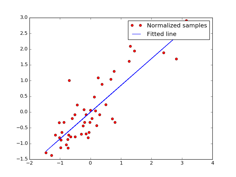
The blue line displays predicted values, using linear regression.
Further reading
- Implementing Logistic and Softmax Regression with TensorFlow
- Basic Concepts and Manipulations with TensorFlow
- Visualizing TensorFlow Graphs with TensorBoard


